
Training and fine-tuning models takes time. During this process it’s important to see progress. This post describes how to visualize output in Tensorboard running locally.
The Hugging Face Trainer API and other machine learning frameworks generate output in Tensorboard format. Tensorboard is often integrated in cloud solutions, but can also be run locally, for example via containers.
Container
The following commands launch Tensorboard in a container. The directory with the logs is mapped in a volume so that data can be copied to or read from this directory from local machines.
1
2
3
4
cd ${Home}
alias docker=podman
docker rm -f tensorboard
docker run -it -p 8888:8888 --name tensorboard -v "$PWD":/tf -p 6006:6006 tensorflow/tensorflow:latest-jupyter
1
2
docker exec -it tensorboard bash
tensorboard --logdir /tf/logs --bind_all
After this the Tensorboard UI and the IPython notebooks UI can be accessed via URLs:
Example
The following example is from the Tensorboard documentation.
1
2
3
4
5
6
7
8
9
10
11
12
13
14
15
16
17
18
19
20
21
22
23
24
25
26
27
28
29
30
31
import tensorflow as tf
import datetime, os

fashion_mnist = tf.keras.datasets.fashion_mnist
(x_train, y_train),(x_test, y_test) = fashion_mnist.load_data()
x_train, x_test = x_train / 255.0, x_test / 255.0

def create_model():
  return tf.keras.models.Sequential([
    tf.keras.layers.Flatten(input_shape=(28, 28), name='layers_flatten'),
    tf.keras.layers.Dense(512, activation='relu', name='layers_dense'),
    tf.keras.layers.Dropout(0.2, name='layers_dropout'),
    tf.keras.layers.Dense(10, activation='softmax', name='layers_dense_2')
  ])

def train_model():
  model = create_model()
  model.compile(optimizer='adam',
                loss='sparse_categorical_crossentropy',
                metrics=['accuracy'])

  logdir = os.path.join("logs", datetime.datetime.now().strftime("%Y%m%d-%H%M%S"))
  tensorboard_callback = tf.keras.callbacks.TensorBoard(logdir, histogram_freq=1)

  model.fit(x=x_train,
            y=y_train,
            epochs=5,
            validation_data=(x_test, y_test),
            callbacks=[tensorboard_callback])

train_model()
The script will produce the following standard output.
1
2
3
4
5
6
7
8
9
10
11
12
13
14
15
16
17
18
Downloading data from https://storage.googleapis.com/tensorflow/tf-keras-datasets/train-labels-idx1-ubyte.gz
29515/29515 [==============================] - 0s 1us/step
Downloading data from https://storage.googleapis.com/tensorflow/tf-keras-datasets/train-images-idx3-ubyte.gz
26421880/26421880 [==============================] - 1s 0us/step
Downloading data from https://storage.googleapis.com/tensorflow/tf-keras-datasets/t10k-labels-idx1-ubyte.gz
5148/5148 [==============================] - 0s 0us/step
Downloading data from https://storage.googleapis.com/tensorflow/tf-keras-datasets/t10k-images-idx3-ubyte.gz
4422102/4422102 [==============================] - 0s 0us/step
Epoch 1/5
1875/1875 [==============================] - 16s 8ms/step - loss: 0.4969 - accuracy: 0.8229 - val_loss: 0.4514 - val_accuracy: 0.8366
Epoch 2/5
1875/1875 [==============================] - 13s 7ms/step - loss: 0.3804 - accuracy: 0.8607 - val_loss: 0.3983 - val_accuracy: 0.8582
Epoch 3/5
1875/1875 [==============================] - 12s 6ms/step - loss: 0.3459 - accuracy: 0.8729 - val_loss: 0.3896 - val_accuracy: 0.8608
Epoch 4/5
1875/1875 [==============================] - 12s 7ms/step - loss: 0.3292 - accuracy: 0.8776 - val_loss: 0.3663 - val_accuracy: 0.8670
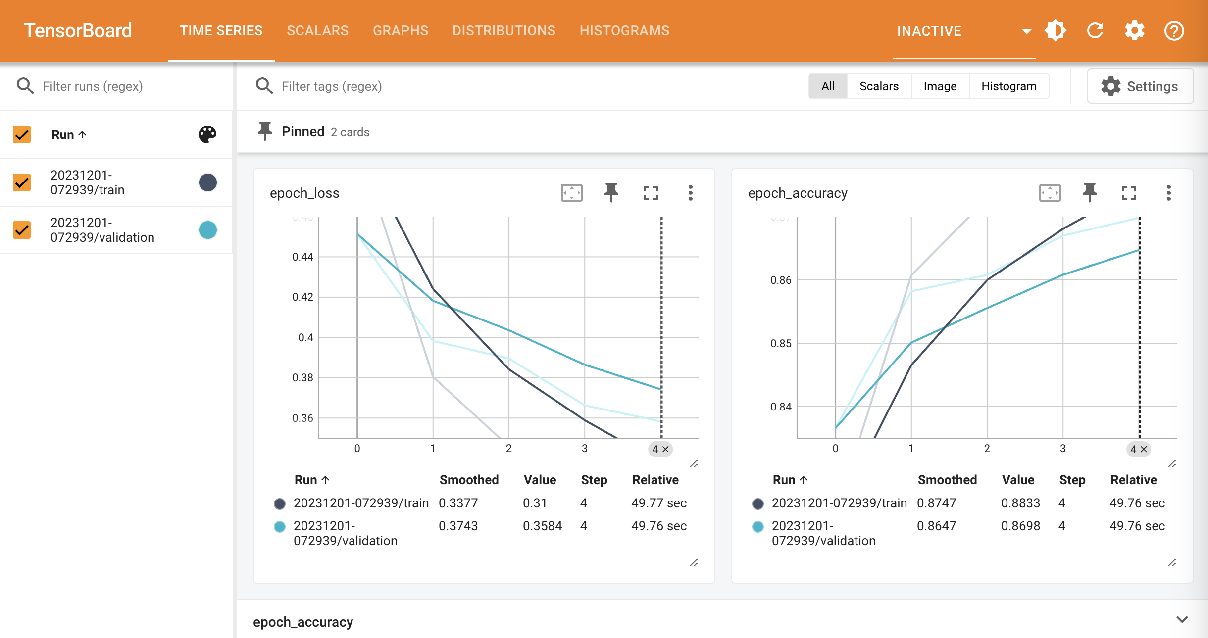
Epoch 5/5
1875/1875 [==============================] - 12s 7ms/step - loss: 0.3100 - accuracy: 0.8833 - val_loss: 0.3584 - val_accuracy: 0.8698
The screenshot at the top shows accuracy and loss in Tensorboard.
Next Steps
To learn more, check out the Watsonx.ai documentation and the Watsonx.ai landing page.